Required section · Section 4 of 6
Working the Analyte X Curve
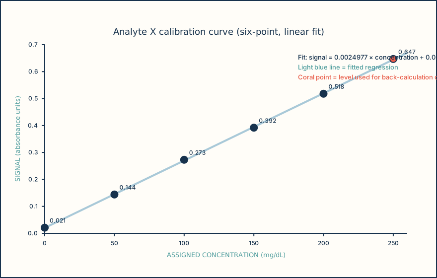
A six-point calibration for a photometric method, Analyte X, reported in mg/dL, runs six calibrators with assigned values of 0, 50, 100, 150, 200, and 250 mg/dL and records an absorbance signal (unitless) for each: 0.021, 0.144, 0.273, 0.392, 0.518, and 0.647. The software fits a first-order linear regression to these six signal-response pairs.
The fitted line is signal = 0.0024977 × concentration + 0.020286. That equation is the working curve: from this point on, every patient specimen's absorbance is converted back to a concentration using this line, until the next calibration.
Back-calculation checks the fit by running each calibrator's own signal back through the equation and comparing the result to its assigned value. At the 250 mg/dL level, the observed signal of 0.647 back-calculates to 250.9 mg/dL, a residual of plus 0.9 mg/dL. At the 0 mg/dL level, the residual is plus 0.3 mg/dL. Across all six points, the residuals scatter between about minus 1.2 and plus 1.2 mg/dL, with no consistent upward or downward trend as concentration increases.
That pattern, small, random scatter around zero with no trend, is what supports accepting this curve. A residual pattern that grows steadily larger at one end, or curves rather than scatters, would instead signal nonlinearity or a proportional bias that a straight-line fit is absorbing into its slope rather than reporting as error, the situation the opening scenario's high-level failure resembles. CLSI EP06 frames this same logic for a full linearity study: judge acceptability from the deviation at each level against a predefined, clinically meaningful limit, not from a summary statistic like R-squared alone, because a high R-squared can coexist with a real, clinically relevant curve or bias.
A good calibration curve is not just a high R-squared, it is small, patternless residuals at every level you checked, including the ones near the edges of the range.
Illustrative drawing — this picture was drawn rather than captured.
| Level (mg/dL) | Observed signal | Fitted signal | Back-calculated (mg/dL) | Residual (mg/dL) |
|---|---|---|---|---|
| 0 | 0.021 | 0.020 | 0.29 | +0.29 |
| 50 | 0.144 | 0.145 | 49.53 | -0.47 |
| 100 | 0.273 | 0.270 | 101.18 | +1.18 |
| 150 | 0.392 | 0.395 | 148.82 | -1.18 |
| 200 | 0.518 | 0.520 | 199.27 | -0.73 |
| 250 | 0.647 | 0.645 | 250.92 | +0.92 |
Knowledge checks
Reading and checks are open. Sign in only to save.
Knowledge check 1
Knowledge check 2
Section status
Finish this section
Reading and checks are open. Sign in only to save.
The module finishes after every required section is marked done and every check in those sections is correct.